Perhaps you would begin by drawing your own continent, or maybe you’d focus on the specific borders of the country you live in. Then, you’d likely move to drawing the outlines of neighboring countries, eventually working your way to far and distant lands. This would be a logical way for anyone to think about such a task, and it gives some insight as to how humans think about the world. We start with what’s familiar, and build it out until it’s a complete picture.
Assembling the World by Economy Size
What if we assembled a world map in a completely different order? Today’s two animations come to us from Engaging-Data, and they approach the world map from an alternate angle: assembling countries on the map in the order of their economic footprints. GDP (Nominal) The first map, shown below, uses nominal GDP to assemble countries in ascending order:
This version of the map shows the smallest economies first, with the larger economies at the end. For this reason, the first economies appearing on the map tend to be developing nations, or nations with smaller geographical or demographic footprints. For example, even though the Falkland Islands are wealthy on a per capita basis, the British Overseas Territory has fewer than 4,000 people, which gives it a minor footprint on a global stage. GDP per Capita (Nominal) Now, let’s take a look at the same map, constructed in order of GDP per capita:
This animation is more cohesive, given that it is not dependent on population size. Instead the order here is based on economic output (in nominal terms) of the average person in each country or jurisdiction. In this case, developing nations appear first – and at the end, more developed regions (like Europe and North America) tend to fill out. Note: All rankings here are in nominal terms, which use market rates to calculate comparable values in U.S. dollars, while omitting the cost of living as a factor. GDP rankings change significantly when using PPP rates.
Other Ways to Assemble the World
While assembling nations based on GDP provides an interesting way to look at the world, this same approach can be tried by applying other statistics as well. We recommend checking out this page, which allows you to “assemble the world” based on measures like population density, life expectancy, or population. on Last year, stock and bond returns tumbled after the Federal Reserve hiked interest rates at the fastest speed in 40 years. It was the first time in decades that both asset classes posted negative annual investment returns in tandem. Over four decades, this has happened 2.4% of the time across any 12-month rolling period. To look at how various stock and bond asset allocations have performed over history—and their broader correlations—the above graphic charts their best, worst, and average returns, using data from Vanguard.
How Has Asset Allocation Impacted Returns?
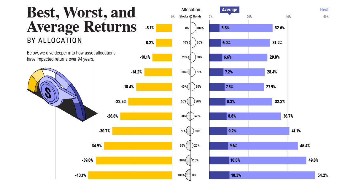
Based on data between 1926 and 2019, the table below looks at the spectrum of market returns of different asset allocations:
We can see that a portfolio made entirely of stocks returned 10.3% on average, the highest across all asset allocations. Of course, this came with wider return variance, hitting an annual low of -43% and a high of 54%.
A traditional 60/40 portfolio—which has lost its luster in recent years as low interest rates have led to lower bond returns—saw an average historical return of 8.8%. As interest rates have climbed in recent years, this may widen its appeal once again as bond returns may rise.
Meanwhile, a 100% bond portfolio averaged 5.3% in annual returns over the period. Bonds typically serve as a hedge against portfolio losses thanks to their typically negative historical correlation to stocks.
A Closer Look at Historical Correlations
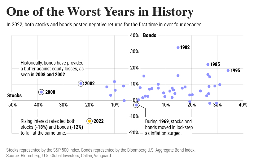
To understand how 2022 was an outlier in terms of asset correlations we can look at the graphic below:
The last time stocks and bonds moved together in a negative direction was in 1969. At the time, inflation was accelerating and the Fed was hiking interest rates to cool rising costs. In fact, historically, when inflation surges, stocks and bonds have often moved in similar directions. Underscoring this divergence is real interest rate volatility. When real interest rates are a driving force in the market, as we have seen in the last year, it hurts both stock and bond returns. This is because higher interest rates can reduce the future cash flows of these investments. Adding another layer is the level of risk appetite among investors. When the economic outlook is uncertain and interest rate volatility is high, investors are more likely to take risk off their portfolios and demand higher returns for taking on higher risk. This can push down equity and bond prices. On the other hand, if the economic outlook is positive, investors may be willing to take on more risk, in turn potentially boosting equity prices.
Current Investment Returns in Context
Today, financial markets are seeing sharp swings as the ripple effects of higher interest rates are sinking in. For investors, historical data provides insight on long-term asset allocation trends. Over the last century, cycles of high interest rates have come and gone. Both equity and bond investment returns have been resilient for investors who stay the course.